Models
この軽音部には問題がある!
Index of Models (Diagonalizable)
Name |
Applications |
Dimension |
TRS |
Parity |
Examples |
|---|---|---|---|---|---|
Rice-Mele Model [Rice1982] |
1+1 |
Spinless |
N/A |
N/A |
|
Rice-Mele Model With Spin [Fu2006] |
1+1 |
Partial |
N/A |
N/A |
|
Su-Schrieffer-Heeger Model [Su1979] |
1 |
Spinless |
N/A |
Polyacetylene |
|
Haldane Model [Haldane1988] |
QAHE |
2 |
Broken |
N/A |
Not yet found [Yu2010] |
Kane-Mele Model [Kane2005] |
2 |
Preserved |
N/A |
Too small in Graphene |
|
BHZ Model [Bernevig2006] |
2D TI |
2 |
Preserved |
Preserved |
HgTe Quantum Well [König2007] |
Thouless Charge Pump (Rice-Mele Model)
Hamiltonian:
\[H = h_{st}(t) \sum_i (-1)^i c^\dagger_i c_i + \frac{1}{2} \sum_{i} \qty[t_0 + (-1)^i \delta(t)] c^\dagger_i c_{i+1} + \mathrm{h.c.}.\]where
\[\begin{split}\delta(t) &= \delta_0 \cos \frac{2\pi t}{T}, \\ h_{st}(t) &= h_0 \sin \frac{2\pi t}{T}.\end{split}\]Bulk Hamiltonian:
\[\begin{split}H = \sum_{k} \begin{pmatrix}a^\dagger_{k} & b^\dagger_{k} \end{pmatrix} \vb{d}\cdot \vb*{\sigma} \begin{pmatrix}a_{k} \\ b_{k} \end{pmatrix},\end{split}\]where
\[\begin{split}d_{x} &= \frac{1}{2} \qty({t_0 + \delta(t)}) + \frac{1}{2}\qty({t_0 - \delta(t)}) \cos k, \\ d_{y} &= -\frac{1}{2} \qty({t_0 - \delta(t)}) \sin k, \\ d_{z} &= h_{st}(t).\end{split}\]Dispersion:
\[E_{\pm} = \pm \abs{\vb{d}}.\]
Fu-Kane Spin Pump (Rice-Mele Model With Spin)
Hamiltonian:
\[H = h_{st}(t) \sum_{i,\sigma} (-1)^i c^\dagger_{i,\sigma} \sigma^z_{\sigma\sigma'} c_{i,\sigma'} + \frac{1}{2} \sum_{i,\sigma} \qty[t_0 + (-1)^i \delta(t)] c^\dagger_{i,\sigma} c_{i+1,\sigma} + \mathrm{h.c.},\]where
\[\begin{split}\delta(t) &= \delta_0 \cos \frac{2\pi t}{T}, \\ h_{st}(t) &= h_0 \sin \frac{2\pi t}{T}.\end{split}\]Bulk Hamiltonian:
\[\begin{split}H = \sum_{k} \begin{pmatrix}\psi^\dagger_{k,\uparrow} & \psi^\dagger_{k,\downarrow} \end{pmatrix} \begin{pmatrix} \vb{d}_+ \cdot \vb*{\sigma} & 0 \\ 0 & \vb{d}_- \cdot \vb*{\sigma} \end{pmatrix} \begin{pmatrix}\psi_{k,\uparrow} \\ \psi_{k,\downarrow} \end{pmatrix},\end{split}\]where
\[\begin{split}\phi^\dagger_{k,\uparrow} &= \begin{pmatrix} a^\dagger_{k,\uparrow} & b^\dagger_{k,\uparrow} \end{pmatrix}, \\ \phi^\dagger_{k,\downarrow} &= \begin{pmatrix} a^\dagger_{k,\downarrow} & b^\dagger_{k,\downarrow} \end{pmatrix}, \\ d_{\pm, x} &= \frac{1}{2} \qty({t_0 + \delta(t)}) + \frac{1}{2}\qty({t_0 - \delta(t)}) \cos k, \\ d_{\pm, y} &= -\frac{1}{2} \qty({t_0 - \delta(t)}) \sin k, \\ d_{\pm, z} &= \pm h_{st}(t).\end{split}\]Dispersion:
\[E_{\pm,\uparrow/\downarrow} = \pm \abs{\vb{d}}.\]
Degeneracy:
Kramers degeneracy: TRS is broken by the on-site term. Kramers degeneracy occurs only at \(t=0\) and \(t=T/2\).
Now comes the most interesting point: for the four states nearest to the Fermi level (two above and two below), we have the following.
At \(t=0\), the first Kramers pair is between the occupied spin-up and spin-down state in the bluk, the second is between the unoccupied pair.
At \(0<t<T/2\), we have no Kramers pair since the TRS is broken.
Caution
We still have two-fold degeneracy here because of the inversion symmetry.
At \(t=T/2\), we have a four-fold degeneracy.
The first Kramers pair is between the occupied spin-up and unoccupied spin-down state on the left end, the second is between the pair on the right end.
The degeneracies are between two different group of bands. Therefore, the bands are guaranteed to cross.
Su-Schrieffer-Heeger Model
Hamiltonian:
\[H = \sum_{n=1}^N (t+\delta t) c_{A,n}^\dagger c_{B,n} + \mathrm{h.c.} + \sum_{n=1}^{N-1} c_{A,n+1}^\dagger c_{B,n} + \mathrm{h.c.}.\]Bulk Hamiltonian:
\[H = \sum_{k} \psi^\dagger_k \qty(d_x \sigma_x + d_z \sigma_z) \psi_k,\]where
\[\begin{split}d_x &= -(t - \delta t), \\ d_z &= 2 \delta t + 2(t - \delta t) \sin^2 \frac{k}{2}, \\ \psi_k &= \begin{pmatrix} a_k \\ b_k \end{pmatrix}.\end{split}\]Dispersion:
\[E_\pm = \pm\sqrt{d_x^2 + d_z^2}.\]
QAHE (Haldane Model)
Hint
Yet to be done.
QSHE (Kane-Mele Model)
Hint
Yet to be done.
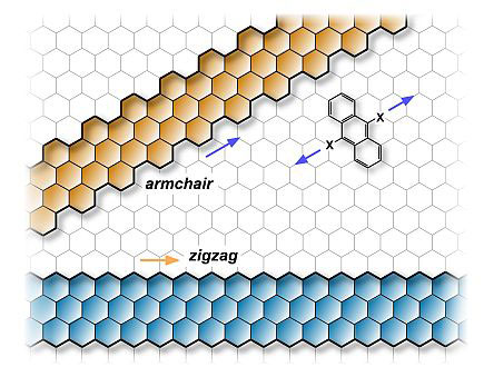
Boundary could be zig-zag, armchair – you name it.
See Kane-Mele Model for bulk band structure.
Bernevig-Hughes-Zhang Model
Got the trick of calculating \(\mathbb{Z}_2\) index? Let hunt down a real beast!
Normal: p orbital below s orbital.
Inverted: p orbital above s orbital due to spin-orbit interaction around \(\vb{k}=0\). This occurs when the \(\ce{HgTe}\) sample is thick enough.
The four orbitals comes into play:
\[\ket{s,\uparrow},\quad \ket{s,\downarrow},\quad \ket{p_x + ip_y,\uparrow},\quad \ket{p_x - ip_y,\downarrow}.\]Hamiltonian:
\[\begin{split}H &= \sum_i \sum_{\alpha=s,p} \sum_{\sigma=\pm} \epsilon_\alpha c^\dagger_{i,\alpha,\sigma} c_{i,\alpha,\sigma} \\ &\phantom{{}={}} -\sum_i \sum_{\alpha=s,p} \sum_{\mu=\pm x,\pm y} \sum_{\sigma=\pm} t^{\alpha\beta}_{\mu\sigma} c^\dagger_{i+\mu, \alpha, \sigma} c_{i,\beta,\sigma},\end{split}\]where
\[\begin{split}t_{\mu \sigma} = \begin{pmatrix} t_{ss} & t_{sp} e^{i\sigma \theta_\mu} \\ t_{sp} e^{-i\sigma \theta_\mu} & -t_{pp} \end{pmatrix},\end{split}\]and \(\theta_\mu\) is the angle between \(\mu\)-direction and \(x\)-axis, taking values \(0\), \(\pi/2\), \(\pi\), \(3\pi/2\).
Bulk Hamiltonian:
\[\begin{split}H &= \sum_{\vb{k}} c^\dagger_{\vb{k}} \qty(\frac{\epsilon_s + \epsilon_p}{2} \mathbb{1}\otimes \mathbb{1} + \frac{\epsilon_s - \epsilon_p}{2}\sigma_z \otimes \mathbb{1}) c_{\vb{k}} \\ &\phantom{{}={}} - \sum_{\vb{k}} c^\dagger_{\vb{k}} \qty[ (t_{ss} - t_{pp}) \sum_\mu (\cos \vb{k} \cdot \vb{a}_\mu) \mathbb{1}\otimes \mathbb{1} + (t_{ss} + t_{pp}) \sum_\mu (\cos \vb{k}\cdot \vb{a}_\mu) \sigma_z \otimes \mathbb{1} + (2 t_{sp} \sin \vb{k} \cdot \vb{a}_1) \sigma_y \otimes \mathbb{1} + (2t_{sp} \sin \vb{k} \cdot \vb{a}_2) \sigma_x \otimes s_z ] c_{\vb{k}},\end{split}\]where \(\vb{a}_1 = \hat{\vb{x}}\) and \(\vb{a}_2 = \hat{\vb{y}}\), and
\[c^\dagger_{\vb{k}} = \begin{pmatrix} c^\dagger_{\vb{k}, s\uparrow} & c^\dagger_{\vb{k}, s\downarrow} & c^\dagger_{\vb{k}, p\uparrow} & c^\dagger_{\vb{k}, p\downarrow} \end{pmatrix}.\]Both \(\sigma_i\) and \(s_i\) denote Pauli matrices.
Simplification: with
\[\begin{split}\Gamma^1 &= \sigma_x \otimes s_x, \\ \Gamma^2 &= \sigma_x \otimes \sigma_y, \\ \Gamma^3 &= \sigma_x \otimes \sigma_z, \\ \Gamma^4 &= \sigma_y \otimes \mathbb{1}, \\ \Gamma^5 &= \sigma_z \otimes \mathbb{1},\end{split}\]we rewrite the Hamiltonian as
\[H(\vb{k}) = d_0(\vb{k}) \mathbb{1} + \sum_{a=1}^5 d_a(\vb{k}) \Gamma^a,\]where
\[\begin{split}d_0(\vb{k}) &= \frac{\epsilon_s + \epsilon_p}{2} - (t_{ss} - t_{pp}) (\cos \vb{k} \cdot \vb{a}_1 + \cos \vb{k} \cdot \vb{a}_2), \\ d_1(\vb{k}) &= 0, \\ d_2(\vb{k}) &= 0, \\ d_3(\vb{k}) &= 2t_{sp} \sin \vb{k} \cdot \vb{a}_2, \\ d_4(\vb{k}) &= 2t_{sp} \sin \vb{k} \cdot \vb{a}_1, \\ d_5(\vb{k}) &= \frac{\epsilon_s - \epsilon_p}{2} - (t_{ss} + t_{pp}) (\cos \vb{k} \cdot \vb{a}_1 + \cos\vb{k}\cdot \vb{a}_2).\end{split}\]Dispersion:
\[E(\vb{k}) = d_0(\vb{k}) \pm \sqrt{\sum_{a=1}^5 d_a(\vb{k})^2}.\]
Parity operator: since \(s\)-orbital has parity \(+1\) and \(p\) orbital has parity \(-1\),
\[\Pi = \sigma_z \otimes \mathbb{1} = \Gamma^5.\]Time-reversal and parity:
\[\begin{split}\Theta \Gamma^a \Theta^{-1} &= \begin{cases} -\Gamma^a, & a = 1,2,3,4, \\ +\Gamma^a, & a = 5. \end{cases} \\ \Pi \Gamma^a \Pi^{-1} &= \begin{cases} -\Gamma^a, & a = 1,2,3,4, \\ +\Gamma^a, & a = 5. \end{cases}\end{split}\]At TRIMs:
\[H(\vb{k} = \Lambda_i) = d_0(\Lambda_i) \mathbb{1} + d_5(\Lambda_i) \Gamma^5.\]The two \(s\)-orbitals are generated, as well the the two \(p\)-orbitals: with \(\ket{\pm}\) denoting parities,
\[\begin{split}H(\Lambda_i) \ket{+} &= \qty[d_0(\Lambda_i) + d_5(\Lambda_i)] \ket{+}, \\ H(\Lambda_i) \ket{-} &= \qty[d_0(\Lambda_i) - d_5(\Lambda_i)] \ket{-}.\end{split}\]
Band inversion: considering half-filled case,
If \(d_5(\Lambda_i) < 0\), the \(-1\) parity is filled, and therefore \(\delta(\Lambda_i) = -1\).
If \(d_5(\Lambda_i) > 0\), the \(+1\) parity is filled, and therefore \(\delta(\Lambda_i) = +1\).
Parity:
\[\delta(\Lambda(n_1, n_2)) = -\operatorname{sign}\qty[\frac{\epsilon_s - \epsilon_p}{2} - (t_{ss} + t_{pp}) \qty{ (-1)^{n_1} + (-1)^{n_2} }].\]
Note
The Hamiltonian is diagonal in the basis we choose only at TRIMs. As we slowing moving from one TRIM to another, the eigenstates are a mixture of both parities in the middle. After we arrive at the ending TRIM, we may surprisingly find that the parity is different from where we begin.
\(\mathbb{Z}_2\) index:
If \(\epsilon_s - \epsilon_p > 4(t_{ss} + t_{pp})\), \(\delta < 0\) for all \(\Lambda_i\) and therefore the system is topologically trivial.
If \(0 < \epsilon_s - \epsilon_p < 4(t_{ss} + t_{pp})\), \(\delta < 0\) for all \(\Lambda_i\) but \(\Lambda(0,0)\), and therefore \(\nu = 1\).
Miscellaneous
A few models that are not mentioned above.
The QWZ (Qi-Wu-Zhang) model. See 二维陈绝缘体(2D Chern Insulator):Qi-Wu-Zhang(QWZ)模型.
See 能带推导复习 - 泰勒猫爱丽丝的文章 - 知乎 for calculation procedures.
See 如何理解量子霍尔效应? - 泰勒猫爱丽丝的回答 - 知乎 for a brief introduction of QSHE.